This series of blogs is to document my application of keras to predict the land values in Melbourne.
The Keras library in Python allows the implementation of neural network/deep learning model easily. For more information, refer to its documentation page. Most resources can be found in Datacamp (where I learnt most of my data science from) and Stackoverflow.
The data set is from Kaggle.
The implementation of Keras is by no means comprehensive. Indeed, it was intended for my own learning and practise.
For my codes and plots, you can refer to my github page here.
The Melbourne Housing Data
The data consists of 19 columns with over 14,000 rows of data. The following screenshot (from Kaggle) summarises the data details.

Obviously, the Price will be the subject of interest. Intuitively, questions that involve the parameters with regard to the price will follow. I have discovered some of them in this exercise, which I am going to share in the next section.
Cleaning the Data
It is observed that there are missing data and outliers. Hence before fully exploring and discovering relationship between the parameters, the data needs to be cleaned.
For the treatment of missing data, I opt to impute the median of the data set, because it is a more reliable measure since there is outliers in the data. I did this by first defining a function, then groupby and transform the data using Pandas:
def impute_median(series):
 return series.fillna(series.median())

df['Landsize'] = df.groupby('Suburb')['Landsize'].transform(impute_median)
For the treatment of outliers, I omitted a value if it is greater than num standard deviations from the mean:
Some missing values, even after imputation, are dropped. This amounts to about 1000 data. Sounds sizeable, but I am left with 13,000+ data, which I think is still about to make a meaningful study.
I have also converted the price to Thousands.
df = df[np.abs((df['Land Price'] - df['Land Price'].mean())) < (num * np.std(df['Land Price']))]
I defined num as 2 in my code. This treatment has to be applied to Building Area, Land Size too.Some missing values, even after imputation, are dropped. This amounts to about 1000 data. Sounds sizeable, but I am left with 13,000+ data, which I think is still about to make a meaningful study.
I have also converted the price to Thousands.
Exploring the Data
The best way to explore the data is through visualisation. Plots group by Suburbs are plotted. However, there are 140+ of them and it is not meaningful to have them in one plot. I'm going to just share a few here. All plots can be found in my github link.
(All plots are plotted using ggplot2 in Python. As you might know, ggplot2 is a popular visualisation package in R.)
Effect of Rooms In Different Suburbs


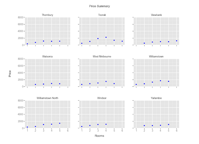 Observations:
1. Some suburbs command higher pay, even for fewer rooms. These are generally closer to the CBD.
2. Prices seems to peak at 4 or 5 rooms, and taper down there after.
(I notice there are data points for 2.5, 3.5 rooms etc. I have to relook at the code to see if there is anything I coded wrongly).
Effect of Landsize and Property Type


Observations:
1. Prices for houses (h) are generally higher. There seem to have no relationship with the houses' price and the landsize.
2. The prices for development site (t) and unit (u) are gneerally insensitive to the land size too.
The best way to explore the data is through visualisation. Plots group by Suburbs are plotted. However, there are 140+ of them and it is not meaningful to have them in one plot. I'm going to just share a few here. All plots can be found in my github link.
(All plots are plotted using ggplot2 in Python. As you might know, ggplot2 is a popular visualisation package in R.)
Effect of Rooms In Different Suburbs


1. Some suburbs command higher pay, even for fewer rooms. These are generally closer to the CBD.
2. Prices seems to peak at 4 or 5 rooms, and taper down there after.
(I notice there are data points for 2.5, 3.5 rooms etc. I have to relook at the code to see if there is anything I coded wrongly).
Effect of Landsize and Property Type


Observations:
1. Prices for houses (h) are generally higher. There seem to have no relationship with the houses' price and the landsize.
2. The prices for development site (t) and unit (u) are gneerally insensitive to the land size too.
Price per unit Landsize Vs Building Area per Landsize
This seems to be quite similar to the previous plots, but this is to explore if bigger buildings (as compared to their land size) will command higher prices. Prices are also normalised to the land size. The property type are also shown in terms of the colour.


Observations:
1) Here, it seems that as long as the building area is large, it is likely to command higher price, regardless of the property type.
Implementing the Model
There are four main steps to implementing the deep neural network using Keras:
1. Define the model architecture
2. Compile the model
3. Fit the model with training dataset
4. Make predictions
Step 1: Define the Model Architecture
The simplest architecture in Keras is the Sequential model. We can define the model by using the following steps:
For the first layer of the model, number of columns of the data needs to be defined via the input_shape argument.
We also need to define the activation function of the layer.
Step 2: Compile the model
Once the model architecture is defined, the model needs to be compiled. The aims of compiling the model are to:
1. specify the optimiser for backpropagation
2. specify the loss function
The optimiser can be customised to determine the learning rate, which is an important component to a neural network.
For classification problem, the loss function is to be defined as 'categorical_crossentropy' and an additional argument metric = ['accuracy'] is added to enable easier assessment of the model.
Now the model is ready for fitting.
Step 3: Fit the model with training dataset
Fitting the model is simply:
The model can be also stopped prematurely if there is no improvement in additional runs (epochs). This can be done by defining a early-stop monitor using the EarlyStopping function, then add a callback argument in the compile method.
Additional points to note: The inputs, namely predictors and target, must be in Numpy arrays. Otherwise there will be errors. If the data is in a pandas dataframe, it can be converted using the as_matrix() method or the .values attribute.
Step 3.5: Saving and Loading the Model
Use the .save() method to save the model. Note that the h5py is required because all models will be saved with the .h5 extension.
To load model, simply:
Now the model can be used to make predictions.
Step 4: Make predictions
There are four main steps to implementing the deep neural network using Keras:
1. Define the model architecture
2. Compile the model
3. Fit the model with training dataset
4. Make predictions
Step 1: Define the Model Architecture
The simplest architecture in Keras is the Sequential model. We can define the model by using the following steps:
import numpy as np
from keras.models import Sequential

model = Sequential()
Now, layers can be added to the models. This can be done by using the .add() method. The simplest architecture will be the Dense architecture where all the nodes between adjacent layers are connected.
For the first layer of the model, number of columns of the data needs to be defined via the input_shape argument.
We also need to define the activation function of the layer.
from keras.layers import Dense
n_cols = predictors.shape[1]
model.add(Dense(100, activation = 'relu', input_shape = n_cols))
model.add(Dense(100, activation = 'relu'))
model.add(Dense(1))
For this model there is one input layer, one hidden layer and one output layer. Here we use the Rectified Linear Activation, ReLU, as the activation function. This functions retuns the value if it is positive, and 0 otherwise.
Step 2: Compile the model
Once the model architecture is defined, the model needs to be compiled. The aims of compiling the model are to:
1. specify the optimiser for backpropagation
2. specify the loss function
The optimiser can be customised to determine the learning rate, which is an important component to a neural network.
model.compile(optimiser = 'adam', loss = 'mean_squared_error')adam is one of the optimisers built in Keras. There are many others optimisers to be used, do check out the documentation for more information.
For classification problem, the loss function is to be defined as 'categorical_crossentropy' and an additional argument metric = ['accuracy'] is added to enable easier assessment of the model.
Now the model is ready for fitting.
Step 3: Fit the model with training dataset
Fitting the model is simply:
model.fit(predictors, target)Cross validation can be performed during the fitting process by defining the validation_split argument.
The model can be also stopped prematurely if there is no improvement in additional runs (epochs). This can be done by defining a early-stop monitor using the EarlyStopping function, then add a callback argument in the compile method.
from keras.callbacks import EarlyStopping
esm = EarlyStopping(patience = 3)

model.fit(predictors, targets, \
validation_split = 0.3, \
epochs = 20, \
callbacks = [esm])
By defining patience = 3, the fitting of the model will stop if there are 3 consecutive epochs with similar performance. Also, the default epochs is 10.
Additional points to note: The inputs, namely predictors and target, must be in Numpy arrays. Otherwise there will be errors. If the data is in a pandas dataframe, it can be converted using the as_matrix() method or the .values attribute.
predictor.as_matrix()
predictor.values
Step 3.5: Saving and Loading the Model
Use the .save() method to save the model. Note that the h5py is required because all models will be saved with the .h5 extension.
import h5py
model.save('model.h5')
To load model, simply:
from keras.models import load_model
my_model = load_model('model.h5')
Now the model can be used to make predictions.
Step 4: Make predictions
To make predictions, simply use the .predict() method.
pred = model.predict(data_to_predict_with)
Evaluating the Model
In this exercise, I used variations configuration and then the mean absolute error (MAE) to assess the models. The results are:
2 Hidden Layers
50 nodes, MAE = 33%
100 nodes, MAE = 24%
200 nodes, MAE = 23%
6 Hidden Layers
200 nodes, MAE = 22%
It appears that the best model (so far) is to use the 2 hidden layer configurations with 200 nodes. Other configurations tend to be not accurate, or computationally expensive (especially with bigger architecture).
The following can be tweaked to improve the model:
1. Change the activation function,
2. Change the optimiser,
3. Determine the best learning rate.
These are left for future exploration.
Learning Points
1. The Keras library is indeed a useful tool to build and prototype a neural network quickly. However, it helps tremendously if one has the background to the neural network. One course I would recommend is the Machine Learning by Andrew Ng.
2. While trying to be ambitious to build a large neural network, I ran into errors. This has to do with the data structure and the computation in the neural network (especially the backpropagation part). I should spend more time studying the basics again.
3. SInce Machine Learning uses much linear algebra and matrix notation (as in Point 1), knowing how to use the Numpy library is important. Indeed, the inputs to the model are to Numpy arrays, as mentioned previously.
Conclusion
This is a good exercise to predict land prices using a neural network. More importantly, I have gained a little more understanding of the Keras library. Also as important, I have learnt how to embed codes in this blogger site :)
Hope you enjoyed reading this as much as I have enjoyed myself working out with Keras and compiling this.
~Huat


