Posting After 2 Years' of Hiatus!

Checked my last post and realise it was dated in 2018. I have not been updating here for more than 2 years!

During this time, I changed my job and am applying my data skills into analysing people. In a cool way, I am a People Analyst now. I will blog about this more.

But the change is not after I brushed up my Statistics and Python skills. I tried to read more about Human Resources. And yes, I wanted to say continuous learning has enabled me some mobility in my career.

I am still learning and re-learning Python almost every day.

I am still passionate in investing, so I will still blog about this. With the Novel Coronavirus happening, I believe there will be much to talk about and opportunities to find.

Till then.

~ZF

[Data Science] Thoughts After Completing Coursera's Deep Learning 5-Course Specialisation

I have just completed Coursera's 5-Course Specialisation in Deep Learning taught by Andrew Ng. I have been looking forward to this Deep Learning course after taking Ng's Machine Learning course, also in Coursera, and learning a little more about Deep Learning.

Course Structure

The specialisation consists of 5 courses:

1. Neural Networks and Deep Learning 

This course introduces Neural Networks and Deep Learning. Since I have taken the Machine Learning course, the first half of the course was not totally new to me. Deep Learning is an neural network on steroids:  more hidden layers, which can be multi-dimensional. The exciting part about this course is I get to code Deep Learning Algorithms by hand using Python and Numpy - no Tensorflow or Keras, yet.

2. Improving Deep Neural Networks: Hyperparameter tuning, Regularisation and Optimization 

One of the powerful features of Deep Nets is the ability to learn complex relationship. However, the compromise to this power is the need for many parameters to the algorithm, or hyperparameters, to tune. This course is specifically for tuning hyper paramters. It can be quite dry. The only respite is when the Ng started to touch on Optimisation algorithms. I find this part very interesting, and I get to understand the workings behind when I type things like opt = AdamOptimizer(...) 

3. Structuring Machine Learning Projects 

This is one of the shorter module, and also another drier one. I shall not describe too much about it. The next two courses are the "specialisations" to the course.

4. Convolutional Neural Networks 

Or CovNets for short. It is used for image recognition (or computer vision). Wonder how a security camera is able to pick up faces, verify objects or identify suspicious articles? It is like the works of CovNets. It took me a while to have a fuzzy understanding of this powerful application of Deep Nets.

5. Sequence Models 

What happens if a time dimension is included into data? The data becomes a time series, or sequences. The Recurrent Neural Network is an application of Deep Nets on time series or sequence data. This is also a short course, but a pretty heavy one. It deals with mostly Natural Language Processing (NLP) and Machine Translation. There is also a side project on Jazz music improvisation, which I find interesting too.

The programming exercises are coded in Python using Jupyter Notebooks. They are interesting! Along the way, there will be some opportunity to use Deep Learning frameworks like Keras and Tensorflow. Keras is a "simpler" but less flexible derivative of Tensorflow, by the way.


Take-Away

The reasons I took this specialisation up are:

1. Deep Learning is a building block of artificial intelligence (AI), a topic which I have grown to be very interested in. I always believe AI is going to provide an opportunity to provide more equity to mankind, if managed properly.
2. My current work involves in analysis tasks which I think can be automated. With the knowledge of Deep Learning, I believe I can implement/build something, or at least a proof-of-concept, AI-ish to improvement work efficiency. If complicated tasks like image recognition, jazz improvisation, and even translation can be accomplished by Deep Learning, I believe my work can benefit from it too; I do not think the work I do is more complicated than what Deep Learning can accomplish, honestly.
3. Well, the name "Andrew Ng" has become somewhat a household name for machine learning.

I gained better understanding in Deep Learning and its related concepts. However I come to realise a few "inconvenient"  aspects of learning from online resources, based on my person experience:

1. In online courses, data are provided - cleaned, transformed and ready to be deployed. In real life, data can be a pain to obtain, let alone clean and validated, which will consume much time.
2. The application of the concepts, however, requires much self-study is needed to learn about using Keras and Tensorflow. This mirrors much in real life. Stackoverflow remains my best friend.

Nevertheless, the learning continues.

~ZF

[Investing] Comparing Dollar-Cost Averaging and Buy-Low-Sell-High (B.Lo.S.Hi) Strategies

In my previous post, I applied dollar-cost averaging (DCA) on Nikko AM STI ETF (G3B) on a 5-year time-frame.

Then a friend showed me an article about the fallacy of dollar-cost averaging.

Indeed, I mentioned in my previous post that dollar-cost averaging depends much on the point where the prices are; if one started low, the accumulation will be fast.

But the result of averaging is not average. At times when prices are low, units accumulation takes place. When prices are high, the additional units also contribute to the total value. Units are the one generating dividends too. In good times (prices are high), dollar-cost averaging suppresses costs. In bad times when prices are low, dollar-cost averaging helps consolidate units.

Dollar-cost averaging is a lazy-man style of investing in auto-pilot. It makes sense if investing costs are low. Obviously, it cannot do better than the Buy-Low-Sell-High (BLoShi) strategy, as I will show later. But the DCA has its merits over the BLoShi too, which I will also share my thoughts later.


DCA Vs BLoSHi. Fight!

I have extracted the maximum data (month) from Yahoo! Finance and coded up the following charts using Python. The hypothetical investing strategy is that I am investing $100 per month since 2009, when G3B debutted into the market.

As shown in the above chart, the average costs increases over time, but the rate of increase slows as time advances because of the large amount of units accumuated (not shown here). The points that are marked with a red 'X' are points when the actual price that is below the average price. These will be points in consideration for the BLoSHi approach.

The BLoShi Approach

In the BLoShi approach, funds are accumulated since the start and maximum units will be bought with all the funds accumulated when the price is below the average price of the DCA method. As shown, there are 5 points that mark this criteria. I shall assume that I enter at only two of these - the first (31-Aug-2011) and the last (31-Jan-2016).

The expected result is that this approach would definitely fare better than the DCA. As we shall analyse in the next chart.


DCA Vs BLoSHi. Performance

The following chart shows compares the value of the units held for the whole period in consideration.

The relevant numbers are:

With DCA,
Total Amount invested = $10,800 

Total Units Bought = 3839 

Total Value = $13,669 

Total Yield = 26.565% 

BLoSHi (Without DCA)
Total Amount invested = $8,400 

Total Units Bought = 3280 

Total Value = $11,678 

Total Yield = 39.027%

Due to the perpertual nature of the DCA, the amount accumulated in DCA is definitely more than the approach without - 600 more units as shown. The costs and holding value will also be higher.

Note that the analysis does not include the dividend yield.


A Simple Principle in Investing

"Buying Low and Selling High" is one of the principles of investing. "Buy a dollar for 50-cents". How low is low and how high is high? There are many metrics to determine that. For the lows, some use the 52-week low to gauge, the same is true for the highs. This form some-sort of a price resistance (I am not a trading pro BTW). Some use moving average over a certain period - if the price is below that MA, buy; if the price is above that MA, sell! Simple enough. Of course there is also the almost-mythical intrinsic value.

We may determine the intrinsic value, but we are able to make a best guess of it. Personally, I would say that numbers that are backed by fundamentals. i.e. there is a basis, is probably the more reliable one, because I cannot find satisfactory answers to question like:"How do we know if the price is going to break the 52-week high (or low)?", "How do we know if the prices will go lower even after falling below the MA?". To the latter question, one way is to keep buying, of course.


The Problem with BLoSHi

BLoSHi seems like a very sound investment strategy, I just wait out for the price to be low enough to buy and sell when the price is high enough. However, the investment strategy is oversimplified. Let's look at the statement again, this time I will italics the key words:

I just wait out for the price to be low enough to buy and sell when the price is high enough.

In essence, there is uncertainty in the price movement and the time. Firstly, I need to determine the price - how low/high is adequately low/high to buy/sell? In the above analysis, it is retrospective. It is easy to pin-point prices that are lower than a certain value (an yearly average, for example) on a historical price chart like the above. Again we can use various metrics (discussed above) to determine the price to buy with some confidence.

Next, when prices are live, and when it shows that the price is trending down after a peak, not many of us will be able to overcome the psychological barrier (fear, that is) or the discipline to buy even if it is near the low that we are waiting for. That is because nobody is certain where the price is going - is it going to bottom out? What if it crash?

Finally, holding out cash to wait out for the price to reach buying-low is not efficient at all. There are much opportunity costs to this approach. In the example above, it is more than 5 years between the two purchases (Aug 2011 and January 2016). Consider the amount that could have been paid out. Assuming that the price remains stable at $2.50, a monthly contribution of $100 will allow me to buy 40 units. In a year I would have accumulated 480 units, and 2400 units in 5 years. If each unit pays out 2% or 0.05cents dividends every year, I would have missed out on $360  of dividends in total, that is more than 3 months' worth of contribution.

With 2% dividend, the yields presented above will be about 29% and 39% for the DCA and Non-DCA cases respectively. As mentioned, the BLoSHi has forgone the compounding effect of any dividends.


Conclusion

Dollar-cost averaging is not a perfect investment strategy. Honestly, in my opinion, it cannot beat the market per se, but it helps to suppress costs when prices are high and accumulate units when prices are low. Here 'highs' and 'lows' are relative to the average price. It also helps one stay invested without the psyhchological barrier when prices dip, and it optimizes the effect of compounding. It also helps negate the need for large capital outlay. This way, we still can get back a fair share from the stock market even though the outcome may not be as stellar as the BLoSHi approach, which I shared that there are many barriers to apply efficiently. However, this is all in the pretext that the investing costs are low.

Perhaps, to optimize the results, one way is to increase the contribution when the prices are low. Maybe I shall leave it for another time.

Do feel free to air your comment!

~ZF

[Data Science] Machine Learning - Part 3, Logistic Regression

In a Classification task, the learning algorithm allocates a number 1 if an instance of the object is to a class (True), and 0 otherwise. When predicting, the outcome will be a number between 1 and 0, which can be interpreted as the probability of the object belonging to a certain class.

The common algorithm to do so is the Logistic Regression. The hypothesis function of algorithm is

\[\hat{y} = \frac{1}{1 + e^{-Z}}\]

known as the sigmoid or logistic function, or the S-curve. $Z$ can also be any function with respect to the features and the corresponding weights, for example, $Z = w_1X_1 +w_2 X_2 + w_3X_3$. In the learning algorithm, the weights, $w_1, w_2, w_3$ are determined through optimization, such as Gradient Descent, of the cost function.

The output of the sigmoid function will always be between 0 and 1, as the chart below shows for $Y = \frac{1}{1 + e^{-Z}}$

I shall apply Logistic Regression on the Iris data set. We can call out the dataset in Scikit-Learn using this code:

from sklearn import datasets 

iris = datasets.load_iris()

The data is a dictionary, so we can see the keys using iris.keys(). There are three species of the flower with 50 instances each. Hence there are 150 instances of data.

Next, the feature and label data, X and y respectively.

X = iris['data'][:, 3:] #petal width 

y = (iris['target']==2).astype(np.int) #1 if Iris-Virginica

As shown, only the petal width will be used to identify if the species is Iris-Virginica in this example.

It is always a good idea to split the data into training and test set randomly. I will split 30% the data as test data (that is 45 instances). This can be done easily using Scikit-Learn:

from sklearn.model_selection import train_test_split 

X_train, X_test = train_test_split(X, test_size = 0.3, random_state = 123) 

y_train, y_test = train_test_split(y, test_size = 0.3, random_state = 123)

 Now, we can apply Logistic Regression on the data!

from sklearn.linear_model import LogisticRegression

model = LogisticRegression()

model.fit(X_train, y_train)

The model's attributes such as the intercept and coefficient can be called out using model.intercept_ and model.coef_ respectively. Note the underscore '_'!

Model Coefficient = [[ 2.17900148]] 

Model Intercept = [-3.67603174]

Hence the model is:
\[\hat{y} = \frac{1}{1+e^{2.179X -3.3676}}\]

We can use the model to make predictions.

pred = model.predict(X_test)

To determine how the model fare, we can use a Confusion Matrix to see the number of right classifications. 

from sklearn.metrics import confusion_matrix 

print(confusion_matrix(y_test, pred))

The confusion matrix will come in a form:

[[ TN, FP]
 [FN, TP] ]

The result will be:

[[28  0]

 [ 2 15]]

Hence,

TP = 15
TN = 28
FP = 0
FN = 2

The rows of the matrix are the True classes; the columns are the Predicted classes. Hence there are 15 + 28 instances where the model classfied correctly (15 True predicted as True, or also known as the True Positive; 28 Negative as Negative, or True Negative).

From the confusion matrix, the True Positive Rate, or Precision, the proportion of positives predicted by the model that are truly positive, can be determined.
\[precision = \frac{TP}{TP + FP}\]

Another useful metrics is the proportion of positive instances that are correctly predicted by the model. This is known as the Recall.
\[recall = \frac{TP}{TP + FN}\]

The precision and recall can be computed using the following code:

from sklearn.metrics import precision_score, recall_score 

print('Precision Score = {:0.3f}'.format(precision_score(y_test, pred))) 

print('Recall Score = {:0.3f}'.format(recall_score(y_test, pred)))

The result:

Precision Score = 1.000 (15/15+0)
Recall Score = 0.882 (15/15+2)

If we were to calculate the accuracy, the instances that were predicted correctly, it will be 33% (15/15+28+2). This is why accuracy is never used in classification tasks.

Here's the graphical representation of the things were carried out.

This marks the end of the Logistic Regression example. The logistic regression learning algorithm is one of the important learning algorithm. It is also frequently used as a building block to understand Artificial Neural Networks, or Neural Nets for short, which I hope to touch on soon.

I hope this has been useful in providing a bigger picture to the Logistic Regression learning algorithm. I have deliberately left out the mathematics behind the learning algortihm because there are many resources that can do a better job than I. By the way, the reference quoted below is awesome!


~ZF

References:

[1] Hands-On Machine Learning with Scikit-Learn and Tensor Flow, Aurelien Geron, O'reilly

[Data Science] Machine Learning - Part 2, Essentials of Machine Learning

In my previous post, I briefly described what machine learning is. I shall attempt to dwell into more (but enough) details in this posts.

As mentioned, machine learning is about deploying algorithms on a computer to apply statistical methods in data analytics. An algorithm is a set of instructions to perform a specific tasks, so a machine learning algorithm is a set of instruction for the computer/programme to learn patterns from a set of given data.

Types of Machine Learning Algorithms

There are many machine learning algorithms. The common ones are:

1. Linear Regression
2. Logistic Regression
3. Nearest Neighbours
4. Support Vector Machines
5. Decision Trees (and Random Forests)
6. Neural Networks
7. Clustering
8. Dimensionality Reduction (e.g. Principle Component Analysis, or PCA)

Supervised and Unsupervised Learning Algorithms

Machine learning algorithms are categorized as supervised learning or unsupervised learning - basically it is data with a known outcome, or labels, for the former (supervised learning) and data without labels for the latter (unsupervised learning).

The outcome of supervised learning is to find a general pattern of the data that validates the labels. Items 1-6 in the list above are supervised learning algorithms.

The outcome of unsupervised learning is to find and group general characteristics within the data. Items 7-8 are unsupervised learning algorithms.


Data Types and Coresponding Objectives

Data can be quantitative (numbers, or measurables on a standard scale), or qualitative (description, or non-measureables because not on a standard scale). Qualitative data is also known as categorical data.

Quantitative data is generally used for projection. For example, what would be next year's sales of a shopping mall be like, given the number of visitors to the shopping mall this year?

Qualitative data is generally used for classification, which can be broken down into two tasks: object verification (if a cat is a cat), and object identification (if an object is a cat).

In practice, the two types of data co-exists. It is unlikely to have a pure data of either form. Thus extra care has to be made to handle data because categorical data is usually assigned a number to represent groups or level, and usually this might give algorithms a false sense of scale if adequate consideration is not taken.


Hypothesis Function

Each machine learning algorithm has an assumption about the data, perhaps except neural networks. This assumptions are normally described as a function, called the hypothesis function. For example, the linear regression assumes linear relationship between the data and the label that we are interested in.

For example, the hypothesis function for linear equation is:
\[\hat{Y} = mX + c\]

By convention, $\hat{Y}$ is the approximation (to the real label, $Y$). It is related to the input data $X$ by $m$ and $c$, the parameters of the model; that is, a different set of $m$ and $c$ yields different value of $\hat{Y}$.

Cost Function

The desired $\hat{Y}$ is one that it is closest to $Y$. This means that $Y - \hat{Y}$ is minimum. Any deviation of $\hat{Y}$ from $Y$ is akin to a costs, hence $Y - \hat{Y}$ is the cost function of the algorithm. However, the mean square error is commonly used as the cost function:
\[\min \frac{1}{m}\sqrt{\sum (Y-\hat{Y})^{2}}\]


Optimization

This can be done by finding the optimal set of $m$ and $c$ to satisfy the above condition. We could have also taken the derivative $\frac{dY}{dX}$  and set it equals to 0 to find the minima or the maxima. However, this is not possible when the dimensions of $X$ increases, meaning there are $X_1, X_2, X_3, ..., X_n$ to be considered, in the case of Multivariate Regression. Fortunately there are optimization algorithms to help us find the optimal set of $m$ and $c$, the most common being Gradient Descent.


An Example

For the set of data given below (Figure 1), we can fit a line (in red) that generalizes the pattern (Figure 2).

Figure 1

Figure 2

We can calculate the gradient $m$ and intercept $c$ by hand in this case to find the equation of the line that generalizes the pattern of the data. Or we can use Python and Scikit-Learn to do so. Here's the code:

import numpy as np
import pandas as pd
import sklearn
from sklearn.linear_model import LinearRegression
lm = LinearRegression()
lm.fit(x, y)
print('The coefficient, m = {}'.format(lm.coef_))
print('The intercept, c = {}'.format(lm.intercept_))

This has the following outputs: $m = 2.03364$ and $c = 2.30736$

Graphically,

Data and the fitted Linear Regression model.

As I have showned, I first deployed the statistical approach - fitting a straight line to a model, and then the computer science approach - run a code to perform Linear Regression. I could have computed the gradient ($m$) and intercept ($c$) manually, using derivatives and all but coding negate the hassle - all in 3 lines of code.

I hope this give some idea about machine learning and also the merits of learning to code. Data analytics gets complicated when the data becomes massive - with multi-dimensions and examples.

Till then~

~ZF

[Investing] What is Dollar-Cost Averaging? A Simulated Example

Suppose you have $100, and you consistently and periodically buy a number of an item that you can afford with the $100.

If the price of the item does not vary much, the number of units that you can will also not vary much.

However, if the price of the item varies from period to period, then you get to buy more when the prices are low, and conversely, less if the prices are higher.

This is the principle of dollar-cost averaging, or DCA, the topic for today.

Let me illustate with some simulation and graphs. For the scenario, I am going to deploy DCA over 20 periods, each period I will spend $100 buy an item with a varying price. Prices are hypothetical and illustration purpose only.


Buy More When Prices Are Low

Well, it is expected to see that the number of units bought at each period is a mirror image of the prices.

What is the overall effect?


A Boring But Stable Cost

A cost that can be potentially lower too. The graph below illustrates.

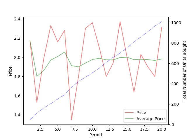
Over a long period, the price of the units will be smoothen out, and at a level that closer to the lows.  Let's see if we extend period to 100 and see the over all effects.

Do you see the average price (green line) seems to be trending down, despite the volatility of prices?

Just for completeness, over a period of 200, the average price does decrease.


Simulated Long Term Performance (Perceived)

This is an update. I reckon it might be useful to see the total value of the investment too.

The graph below shows the overall performance over period = 100.

For a period 100 timeline, the total amount invested is $10,000, as shown by the green line. As time proceeds, the number of units increases, and the overall portfolio value becomes more sensitive to the price. Nevertheless, we can see that there is a potential to exceed the invested value.

In this simulation, prices are made volatile intentionally. If an investor invests in an index funds, the prices should be more stable; he should do better the simulated case.

Last point, the simularion also shows that one should not invest in a stock whose price is so volatile; that is not the intent of the DCA to make the movement of the portfolio value like a roller-coaster ride.


Benefits of DCA

However, the simulation is based on random number generation. In the market, while this kind of price movement is not uncommon, prices are generally cyclical. Nevertheless, I am confident that this little simulation of mine iterates some very important feature of DCA.

1. The DCA is a great tool for long (very long, might I add) positions - it reduces the capital outlay, smoothens out risks and it is investing on auto-pilot. 
2. It is especially good for investing in index funds, or ETFs that track an index, such as the STI, the STI ETF.
3. It is good for discipline i investing. Many options are available in the form of a regular savings plan (RSP), such as the POSB Invest-Saver.*

*This is not an endorsement or recommendation for any investment products

But...

The DCA is not without flaws. In sustained bullish periods, the number of units that can be bought diminishes, until prices drop, and this makes the performance of the previous purchase look extraordinarily bad. You can see this in the graph above, the first few periods where there is a spike is akin to this situation. This should not be too much of a concern though if the investor is going very long. One can simply increase the principle to invest when prices are lower to avert this situation though, but the question remains - how low is low?

One of the golden rule in investing is to keep invested. DCA is one of those tools that can help the investor to do so.

Feel free to comment!

~ZF

P/S: Simulations are performed and plotted using Python.


Afternote: I shall attempt to do a simualtion with real data soon.

[Data Science] So I Have Just Completed the Applied Data Science with Python Specialisation by University of Michigan in Coursera

This specialisation comprises of 5 courses:

Course 1 - Introduction to Data Science in Python
Course 2 - Applied Plotting,  Charting & Data Representation in Python
Course 3 - Applied Machine Learning in Python
Course 4 - Applied Text Mining in Python
Course 5 - Applied Social Network Analysis in Python

I shall summarise what I think about the course:

The Good:

1) The course is structured very well and the pace manageable.

2) All exercises are done and submitted in Jupyter notebookes and graded rather quickly. 

3) Exercises are challenging. Learners have to do much research (through Stack Overflow forums) and the toolkit's documentation pages. 

4) Personally, I learned more about Pandas and Numpy and also performing neural networks using Scikit-Learn MLP (stands for multi-layer perceptron) module.

The Bad:

1) While the course is structured, the materials are administered quickly. It is iterated many times that it is an applied course, and hence much of the intuition behind the methods were just introduced quckly.  

2) Stack Overflow, Stack Overflow.... 

3) The assignment grading can be buggy, and with no expected answers provided, the learner just have to submit and see if they passed. I think such is life as a data scientist? We never know if we get the correct answers. So I suppose that is intent? But much time is wasted just by waiting. 

4) Nothing to do with the course, but I do not quite like the Coursera charging a fee monthly instead of a lump sum. This makes the course very costly in the long run. For example, if this course has 5 modules and presumably each module is a mths's of content, it will cost well above USD$200 to get the specialization. Of course there is an option to just audit the courses.

Who Should Take This Course:

I think this is a course worth taking, afterall the University of Michigan is not a trivial name, but perhaps not spent too much lingering on. So I think it is best to learn the basics of Python, data science and machine learning throught other more cost-effective (by which, I mean cheaper) means.

Here are what I would recommend:

For Python/Data Science

1) I find the book Automate the Boring Stuff with Python is a good start, although I discovered this rather late. This book introduces all the basic programming in Python, such as creating functions, iterations, and also more advanced stuff like reading and automating spreadsheets, webcrawling, and generally automating work using Python. It is easy to read and follow, and the digital copy of the book is free to browse at the link provided.   

2) Jose Portilla's courses pertaining to Python and Data Science in Udemy is an excellent introduction to the subject. And with the constant barrage of sales and offer at Udemy (recently they have a $10 to all courses, for example), it is good to buy and learn at your own pace. I have personally done the Data Science and Machine Bootcamp with Python (and also SQL and R). He also have a Python bootcamp.  

3) Other resources such as Datacamp and Codeacademy is a good place to consider too. Personally, I started Python and R at Codeacademy and Datacamp respectively.

For Machine Learning

1) The videos based on the book An Introduction to Statistical Learning with Applications in R is an must-watch if you wish to have a deeper understanding in the intuition behind the machine learning algorithms, in a statistician point-of-view. It also covers more advanced methods such as Support Vector Machines. However, it does not cover neural networks. Statistical Learning is the statistician way of saying Machine Learning.

2) Andrew Ng has become the household name for Machine Learning. His Machine Learning course in Coursera is becoming a classic. This course approaches Machine Learning in the Computer Science's POV and Andrew is able to explain difficult concepts easy to understand in his softspoken manner. The assignment is challenging and it is in Matlab or Octave. It is this course that I finally appreciate the wonders of matrix algebra (and yes, I am not shy to say I am an engineer). I am currently auditing his Deep Learning course, also in Coursera.


Currently I am still looking for opportunities to use what I have learnt at work (or new opportunities). I am using Python to scrape stock data and am devising a project to scrape financial report data for REIT analysis. More on this in future blogs.

~yZhifa

[Data Science] Whatever I Know About Data Science

Data Science is the subject of gathering insights from data. Yes, it is a fancy name for Statistics.

However, it seems to me that Data Science is commonly interpreted it as the hybrid of two subjects: Data Analysis and Computer Science, and the weight for the latter seems to be heavier. I will share why I think it is so.

You see, much of what that has to be accomplished in data science is by a computer.

Probability and statistical tools such Student t-Test, Chi-Square Test, that are required in data analysis, can be easily computed using software such as R - no more computing of t- (or z-) score then refer to a table. 

Data visualisation is also made easy by using R's ggplot2 or Python's matplotlib or seaborn - there is no need to draw graphs and scale by hand.

Not forgetting data manipulation and transformation. These can be done easily by using Python or R too.

However, let's not forget the ultimate aim of data science - that is to gather insights from the data. Hence a data scientist has to be good in both - programming and statistics. I opine that he does not need to be overly good with programming, just enough to gather, clean, manipulate and analyse the data. But I would place more emphasis on the statistics part because it is statistics that will allow the data scientist to quantify the findings.

Here I list the resource I learnt from.


Statistics

As an engineer, I learnt statistics from JC till University. Also, my Master's degree in Industrial and Systems Engineering is heavy on statistics, although I do not think my statistics is very strong.

Nevertheless here are the resources:

• Statistics for Experimenters: My lecturer sweared by it because it is written by legends. This book is so classic that it only has two revisions, but it is easy to read because the concepts are delivered in real and relatable experiments. 
• Applied Statistics and Probility for Engineers. This is another textbook, more like a supplement to my course.  
• The site Seeing Theory - A visual introduction to probability and statistics is a cool site to learn about the topic graphically. 

In short: basically any probability and statistics textbook or resource that you can get a hold on. The ones I listed are the those I used.


Programming

I had exposure to R because my master course was very statistics-orientated.  R is free and open source and has a big community supporting it, and it does the work. SPSS and SAS are simply too expensive to be accessible in my opinion. One of my lecturers used R to do bootstrapping and it got me interested to want to learn more, and I had been wanting to learn a programming language. R seems to fit the bill. Hence my inclination is towards R when it comes to data science.

I learnt R mainly from DataCamp, and tons of trial and error. You have to pay, a subscription, which I did,  if you wish to access the more in-depth courses. Otherwise, the free way is to learn R in R using SWIRL. R also has a resource to learn probability and statistics, aptly called Introduction to Probability and Statistics Using R (IPSUR). RStudio, and along with it Shiny and RMarkdown, is a powerful IDE for R.

I got to know Python along the way while researching on R and Data Science.  I started learning the basic syntax from Codeacademy. Thereafter I learn from courses in Udemy. The Python for Data Science and Machine Learning in Udemy is especially a good primer to learn data science in Python. i discovered that Python is a very easy language to learn. Compared to R, its syntaxes are more elegant. Also it is more versatile when it comes to big data, and it is able to be integrated with other languages/applications.

To really learn Python to be functional, that is able to write functional scripts, I would recommend the book Automate the Boring Stuffs. I have also read many books on Python such as Python for Data Science for Dummies, and Python Programming for the Absolute Beginner.

I also got to know about Kaggle and KDnuggets. Both are very good sites to browse for data science related information.


Machine Learning

I will regard machine learning as a computer science subject although the statistical counterpart is call statistical learning. Anyway, statistical learning are normally implemented using a computer and therefore machine learning is a more familiar term.

Machine learning is basically using a computer to identify patterns and then make predictions, without the hard coding the logic. In a way it seems like the machine learns about the data. It is a broad but interesting topic.

I would strongly recommend these two resources:

• The video lectures on the book, An Introduction to Statistical Learning with Applications in R, by the authors of the book, who are Stanford University professors. Sit through the 15hours worth of lectures. It is worth it.
• Andrew Ng's Machine Learning Course in Coursera. Coursera, founded by Ng, has a wealth of courses. However, his own course is the must-go to for machine learning. I paid for the certification and it is worth it.

Projects

I think the fastest way to learn is to really do it hands-on. Sure the courses and all will have exercises and assignments, but I do not think it is enough. I would pick up data sets that I think it would be interesting to analyse, and or I have certain personal project that I wish to implement in a programme.

I have:

• Attempted analyse Melbourne's land prices data from Kaggle and made predictions using Keras in Python
• Visualised land value in different areas in Singapore
• Wrote a Python script to scrape stock data and select stocks based on Formula Investing Methodology

Continuous Learning

Well, my reading never stops. These are the books that are in the queue:

• Data Analysis and Graphics Using R
• Machine Learning for Predictive Data Analytics
• Modelling Techniques in Predictive Analytics with Python and R
• Data-ism
• Algorithms to Live By

But I am not a Data Scientist, yet.

~Huat

[Data Science] Predicting Melbourne's Land Value Using Deep Learning

This series of blogs is to document my application of keras to predict the land values in Melbourne.

The Keras library in Python allows the implementation of neural network/deep learning model easily. For more information, refer to its documentation page. Most resources can be found in Datacamp (where I learnt most of my data science from) and Stackoverflow.

The data set is from Kaggle.

The implementation of Keras is by no means comprehensive. Indeed, it was intended for my own learning and practise. 

For my codes and plots, you can refer to my github page here.

The Melbourne Housing Data

The data consists of 19 columns with over 14,000 rows of data. The following screenshot (from Kaggle) summarises the data details.

Obviously, the Price will be the subject of interest. Intuitively, questions that involve the parameters with regard to the price will follow. I have discovered some of them in this exercise, which I am going to share in the next section.

Cleaning the Data

It is observed that there are missing data and outliers. Hence before fully exploring and discovering relationship between the parameters, the data needs to be cleaned.

For the treatment of missing data, I opt to impute the median of the data set, because it is a more reliable measure since there is outliers in the data. I did this by first defining a function, then groupby and transform the data using Pandas:

def impute_median(series):
 return series.fillna(series.median())

df['Landsize'] = df.groupby('Suburb')['Landsize'].transform(impute_median)

For the treatment of outliers, I omitted a value if it is greater than num standard deviations from the mean:

df = df[np.abs((df['Land Price'] - df['Land Price'].mean())) < (num * np.std(df['Land Price']))]

I defined num as 2 in my code. This treatment has to be applied to Building Area, Land Size too.

Some missing values, even after imputation, are dropped. This amounts to about 1000 data. Sounds sizeable, but I am left with 13,000+ data, which I think is still about to make a meaningful study.

I have also converted the price to Thousands.

Exploring the Data

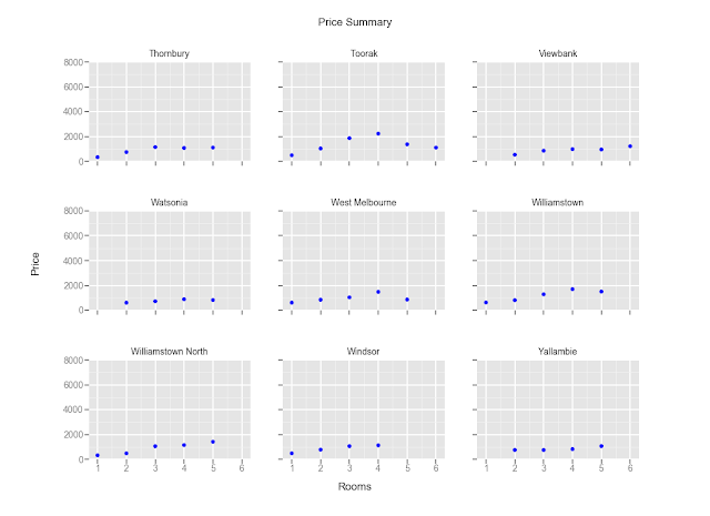
The best way to explore the data is through visualisation. Plots group by Suburbs are plotted. However, there are 140+ of them and it is not meaningful to have them in one plot. I'm going to just share a few here. All plots can be found in my github link.

(All plots are plotted using ggplot2 in Python. As you might know, ggplot2 is a popular visualisation package in R.)


Effect of Rooms In Different Suburbs

Observations:
1. Some suburbs command higher pay, even for fewer rooms. These are generally closer to the CBD.
2. Prices seems to peak at 4 or 5 rooms, and taper down there after.

(I notice there are data points for 2.5, 3.5 rooms etc. I have to relook at the code to see if there is anything I coded wrongly).

Effect of Landsize and Property Type

Observations:
1. Prices for houses (h) are generally higher. There seem to have no relationship with the houses' price and the landsize.
2. The prices for development site (t) and unit (u) are gneerally insensitive to the land size too.

Price per unit Landsize Vs Building Area per Landsize

This seems to be quite similar to the previous plots, but this is to explore if bigger buildings (as compared to their land size) will command higher prices. Prices are also normalised to the land size. The property type are also shown in terms of the colour.

Observations:
1) Here, it seems that as long as the building area is large, it is likely to command higher price, regardless of the property type.

Implementing the Model

There are four main steps to implementing the deep neural network using Keras:
1. Define the model architecture
2. Compile the model
3. Fit the model with training dataset
4. Make predictions



Step 1: Define the Model Architecture

The simplest architecture in Keras is the Sequential model. We can define the model by using the following steps:

import numpy as np
from keras.models import Sequential

model = Sequential()

Now, layers can be added to the models. This can be done by using the .add() method. The simplest architecture will be the Dense architecture where all the nodes between adjacent layers are connected.

For the first layer of the model, number of columns of the data needs to be defined via the input_shape argument.

We also need to define the activation function of the layer.

from keras.layers import Dense
n_cols = predictors.shape[1]
model.add(Dense(100, activation = 'relu', input_shape = n_cols))
model.add(Dense(100, activation = 'relu'))
model.add(Dense(1))

For this model there is one input layer, one hidden layer and one output layer. Here we use the Rectified Linear Activation, ReLU, as the activation function. This functions retuns the value if it is positive, and 0 otherwise.


Step 2: Compile the model

Once the model architecture is defined, the model needs to be compiled. The aims of compiling the model are to:
1. specify the optimiser for backpropagation
2. specify the loss function

The optimiser can be customised to determine the learning rate, which is an important component to a neural network.

model.compile(optimiser = 'adam', loss = 'mean_squared_error')

adam is one of the optimisers built in Keras. There are many others optimisers to be used, do check out the documentation for more information.

For classification problem, the loss function is to be defined as 'categorical_crossentropy' and an additional argument metric = ['accuracy'] is added to enable easier assessment of the model.

Now the model is ready for fitting.


Step 3: Fit the model with training dataset

Fitting the model is simply:

model.fit(predictors, target)

Cross validation can be performed during the fitting process by defining the validation_split argument.

The model can be also stopped prematurely if there is no improvement in additional runs (epochs). This can be done by defining a early-stop monitor using the EarlyStopping function, then add a callback argument in the compile method.

from keras.callbacks import EarlyStopping
esm = EarlyStopping(patience = 3)

model.fit(predictors, targets, \
validation_split = 0.3, \
epochs = 20, \
callbacks = [esm])

By defining patience = 3, the fitting of the model will stop if there are 3 consecutive epochs with similar performance. Also, the default epochs is 10.

Additional points to note: The inputs, namely predictors and target, must be in Numpy arrays. Otherwise there will be errors. If the data is in a pandas dataframe, it can be converted using the as_matrix() method or the .values attribute.

predictor.as_matrix()
predictor.values

Step 3.5: Saving and Loading the Model

Use the .save() method to save the model. Note that the h5py is required because all models will be saved with the .h5 extension.

import h5py
model.save('model.h5')

To load model, simply:

from keras.models import load_model
my_model = load_model('model.h5')

Now the model can be used to make predictions.



Step 4: Make predictions

To make predictions, simply use the .predict() method.

pred = model.predict(data_to_predict_with)

Evaluating the Model

In this exercise, I used variations configuration and then the mean absolute error (MAE) to assess the models. The results are:

2 Hidden Layers
50 nodes, MAE = 33%
100 nodes, MAE = 24%
200 nodes, MAE = 23%

6 Hidden Layers
200 nodes, MAE = 22%

It appears that the best model (so far) is to use the 2 hidden layer configurations with 200 nodes. Other configurations tend to be not accurate, or computationally expensive (especially with bigger architecture).

The following can be tweaked to improve the model:
1. Change the activation function,
2. Change the optimiser,
3. Determine the best learning rate.

These are left for future exploration.

Learning Points

1. The Keras library is indeed a useful tool to build and prototype a neural network quickly. However, it helps tremendously if one has the background to the neural network. One course I would recommend is the Machine Learning by Andrew Ng.

2. While trying to be ambitious to build a large neural network, I ran into errors. This has to do with the data structure and the computation in the neural network (especially the backpropagation part). I should spend more time studying the basics again.

3. SInce Machine Learning uses much linear algebra and matrix notation (as in Point 1), knowing how to use the Numpy library is important. Indeed, the inputs to the model are to Numpy arrays, as mentioned previously.

Conclusion

This is a good exercise to predict land prices using a neural network. More importantly, I have gained a little more understanding of the Keras library. Also as important, I have learnt how to embed codes in this blogger site :)

Hope you enjoyed reading this as much as I have enjoyed myself working out with Keras and compiling this.

~Huat

[Data Science] Embedding Python Codes in Blogger Using SyntaxHighlighter

You know, I have been rendering my R codes to a html files in R Markdown (RMD), then copied the whole HTML codes to paste into blogger.

What I needed was to embed code snippets.

I came across this awesome post to do just that, using SyntaxHighlighter, credit goes to the blogger and the creator of SyntaxHighlighter. And not forgetting StackOverflow.

Here's an example:

import numpy as np
import pandas as pd
import matplotlib.pyplot as plt
import seaborn as sns
import h5py

Now it's a success! Now I can share my data science stuffs here with proper code snippets!

Yay~

Here are the details of setting it up, as some of the steps in the links mentioned are outdated:

In Blogger:

1. Go to Template > Edit HTML (it is a small icon below the blog preview).

2. Copy and paste these codes immediately after the <head> tag:

<script src='http://alexgorbatchev.com/pub/sh/2.1.364/scripts/shCore.js' type='text/javascript'></script>
<script src='http://alexgorbatchev.com/pub/sh/2.1.364/scripts/shBrushPython.js' type='text/javascript'></script>
<link href='http://alexgorbatchev.com/pub/sh/2.1.364/styles/styles/shCore.css' rel='stylesheet' type='text/css' />
<link href='http://alexgorbatchev.com/pub/sh/2.1.364/styles/shThemeDefault.css' rel='stylesheet' type='text/css' />

(In the link provided, the quotation marks in the links are presented as '&#x27;' - Blogger does not accept it)

3. Save the template.

4. Go to Layout.

5. Add a HTML/Javascript Gadget - Any location will do. I chose one at the side bar.

6. Add a title for the gadget. Remember this title because you have to locate it later in the HTML code in order to hide the gadget. Use SyntaxHighlighter if you can't think of one.

7. In the content box, include this code:

<script class='javascript'>//<![CDATA[
SyntaxHighlighter.config.clipboardSwf = 'http://alexgorbatchev.com/pub/sh/2.1.364/scripts/clipboard.swf';
SyntaxHighlighter.all();
//]]></script>

8. Save the gadget.

9. Now, head back to Template > Edit HTML. Locate the widget id of the gadget you just added in. It can be found within the b:widget tag. (It is HTML1 for me.)

10. Locate the <b:skin> ... </b:skin>. Expand it and before the ]]></b:skin>, include this code to hide the gadget:

#HTML1 {display:none;}

11. Save the template and all is good to go!

Note: Somehow it does not work in Preview.


~Huat